TidyTuesday - The Tate Collection

Last week's #TidyTuesday. Had something very specific in mind & it forced me to learn a new pkg and some base R to finish this plot.

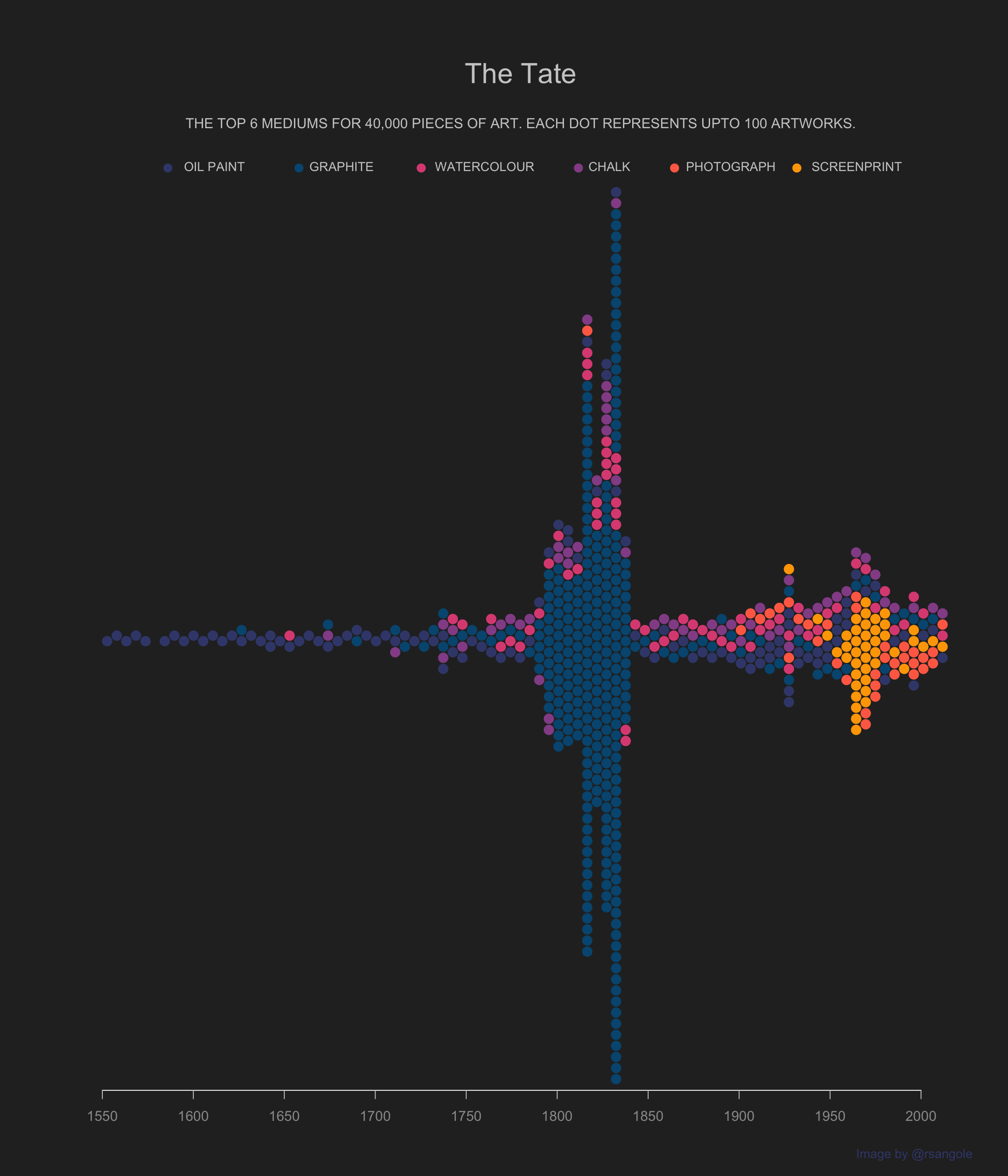
I wanted to showcase the change in the dominant medium from Graphite to Screenprint, which we can see in this beeswarm plot.#rstats pic.twitter.com/6uMCLHag4P

— Rahul (@rsangole) January 20, 2021

library(tidyverse)
library(tidyr)
library(data.table)
library(beeswarm)
library(extrafont)
# extrafont::font_import(paths = ".", prompt = F)

artists <- data.table::fread("artists.csv") %>% 
  mutate(gender = ifelse(is.na(gender), "Unknown", gender),
         gender = factor(gender,levels = c("Male","Female", "Unknown"), ordered = TRUE),
         life_yr = yearOfDeath - yearOfBirth,
         pre_1850 = yearOfBirth < 1850,
         name_len = stringr::str_length(name) - 2) %>% 
  separate(col = "placeOfBirth", sep = ",", into = c("birth_city", "birth_country"), remove = F) %>% 
  separate(col = "placeOfDeath", sep = ",", into = c("death_city", "death_country"), remove = F) %>% 
  mutate(moved_countries = birth_country != death_country,
         birth_country = ifelse(is.na(birth_country), "Unknown", birth_country),
         death_country = ifelse(is.na(death_country), "Unknown", death_country))
artwork <-
    data.table::fread("artwork.csv") %>%
    mutate(
        artistRole = as.factor(artistRole),
        medium = as.factor(medium),
        units = as.factor(units),
        area = width * height,
        title_len = stringr::str_length(title)
    ) %>%
    left_join(
        y = artists %>% select(name, gender, yearOfBirth, birth_city, birth_country, life_yr),
        by = c("artist" = "name")
    )


color_pallete <- c("#005780",
                   "#3e487a",
                   "#955196",
                   "#dd5182",
                   "#ff6e54",
                   "#ffa600")

artwork[,
        medium_cleaned := case_when(
            grepl(pattern = "Graphite", x = medium) ~ "Graphite",
            grepl(pattern = "Oil paint", x = medium) ~ "Oil Paint",
            grepl(pattern = "Screenprint", x = medium) ~ "Screenprint",
            grepl(pattern = "Watercolour", x = medium) ~ "Watercolour",
            grepl(pattern = "photograph|Photograph", x = medium) ~ "Photograph",
            grepl(pattern = "chalk|Chalk", x = medium) ~ "Chalk"
        )]
artwork[,
        color := case_when(
            medium_cleaned %like% "Graphite" ~ color_pallete[1],
            medium_cleaned %like% "Paint" ~ color_pallete[2],
            medium_cleaned %like% "Screenprint" ~ color_pallete[6],
            medium_cleaned %like% "Watercolour" ~ color_pallete[4],
            medium_cleaned %like% "Photograph" ~ color_pallete[5],
            medium_cleaned %like% "Chalk" ~ color_pallete[3]
        )]
medium_dat_2 <- artwork[, .(year, medium_cleaned, color)]

bees_plot <- medium_dat_2 %>%
    filter(!is.na(medium_cleaned), !is.na(year)) %>%
    arrange(year)
bees_plot[, cutpts_numeric := cut(year, breaks = seq(1500, 2015, 5), labels = F)]
bees_plot[, cutpts := cut(year, breaks = seq(1500, 2015, 5))]
bees_plot[, xaxis := as.numeric(substr(cutpts, 2, 5))]

bees_plot_reduced <-
    bees_plot[, .N, .(xaxis, medium_cleaned, color, cutpts_numeric)]
bees_plot_reduced[, num_pts := ceiling(N / 100)]

datlist <- list()
for (i in 1:nrow(bees_plot_reduced)) {
    .nrows = bees_plot_reduced[i, num_pts]
    .dlist <- list()
    for (j in 1:.nrows) {
        .dlist[[j]] <-
            bees_plot_reduced[i, .(xaxis, medium_cleaned, color, cutpts_numeric)]
    }
    datlist[[i]] <- rbindlist(.dlist)
}

to_plot <- rbindlist(datlist)
glimpse(to_plot)

Rows: 624
Columns: 4
$ xaxis          <dbl> 1540, 1555, 1560, 1565, 1570, 1575, 1585, 1590, 1595, 1…
$ medium_cleaned <chr> "Oil Paint", "Oil Paint", "Oil Paint", "Oil Paint", "Oi…
$ color          <chr> "#3e487a", "#3e487a", "#3e487a", "#3e487a", "#3e487a", …
$ cutpts_numeric <int> 9, 12, 13, 14, 15, 16, 18, 19, 20, 21, 22, 23, 24, 25, …

make_plot <- function(to_plot) {
    categories <- unique(to_plot[, .(medium_cleaned, color)])
    xleg <- c(1.0,  2.8,  4.6,  6.8,  8.2, 10.0)
    beeswarm(
        xleg,
        pwcol = categories$color,
        horizontal = TRUE,
        method = "center",
        cex = 1.3,
        pch = 19,
        xlim = c(0, 12),
        axes = FALSE
    )
    text(
        x = xleg + 0.05,
        y = 1,
        labels = toupper(categories$medium_cleaned),
        col = "gray80",
        pos = 4,
        cex = 0.9
    )
}
make_plot_2 <- function(to_plot) {
    beeswarm(
        x = to_plot$xaxis,
        pwcol = to_plot$color,
        horizontal = TRUE,
        method = "hex",
        spacing = 1.1,
        cex = 1.5,
        pch = 19,
        xlim = c(1550, 2010),
        axes = FALSE
    )
    x <- seq(from = 1550, to = 2000, by = 50)
    axis(
        side = 1,
        labels = x,
        at = x,
        col = "white",
        col.ticks = "gray80",
        col.axis = "gray60"
    )
}
par(
    fig = c(0, 1, 0.7, 1),
    new = TRUE,
    bg = "#292929"
    # family = "Monoid"
)
make_plot(to_plot = to_plot)
par(fig = c(0, 1, 0, 0.9), new = TRUE)
make_plot_2(to_plot = to_plot)
mtext(
    text = "The Tate",
    side = 3,
    cex = 2,
    col = "gray80",
    padj = -5
)
mtext(
    text = "THE TOP 6 MEDIUMS FOR 40,000 PIECES OF ART. EACH DOT REPRESENTS UPTO 100 ARTWORKS.",
    side = 3,
    cex = 1,
    col = "gray80",
    padj = -5.5
)
mtext(
    text = "Image by @rsangole",
    side = 1,
    cex = 0.9,
    col = "#3e487a",
    padj = 6,
    adj = 1
)