Visualizing Correlations
Visualization
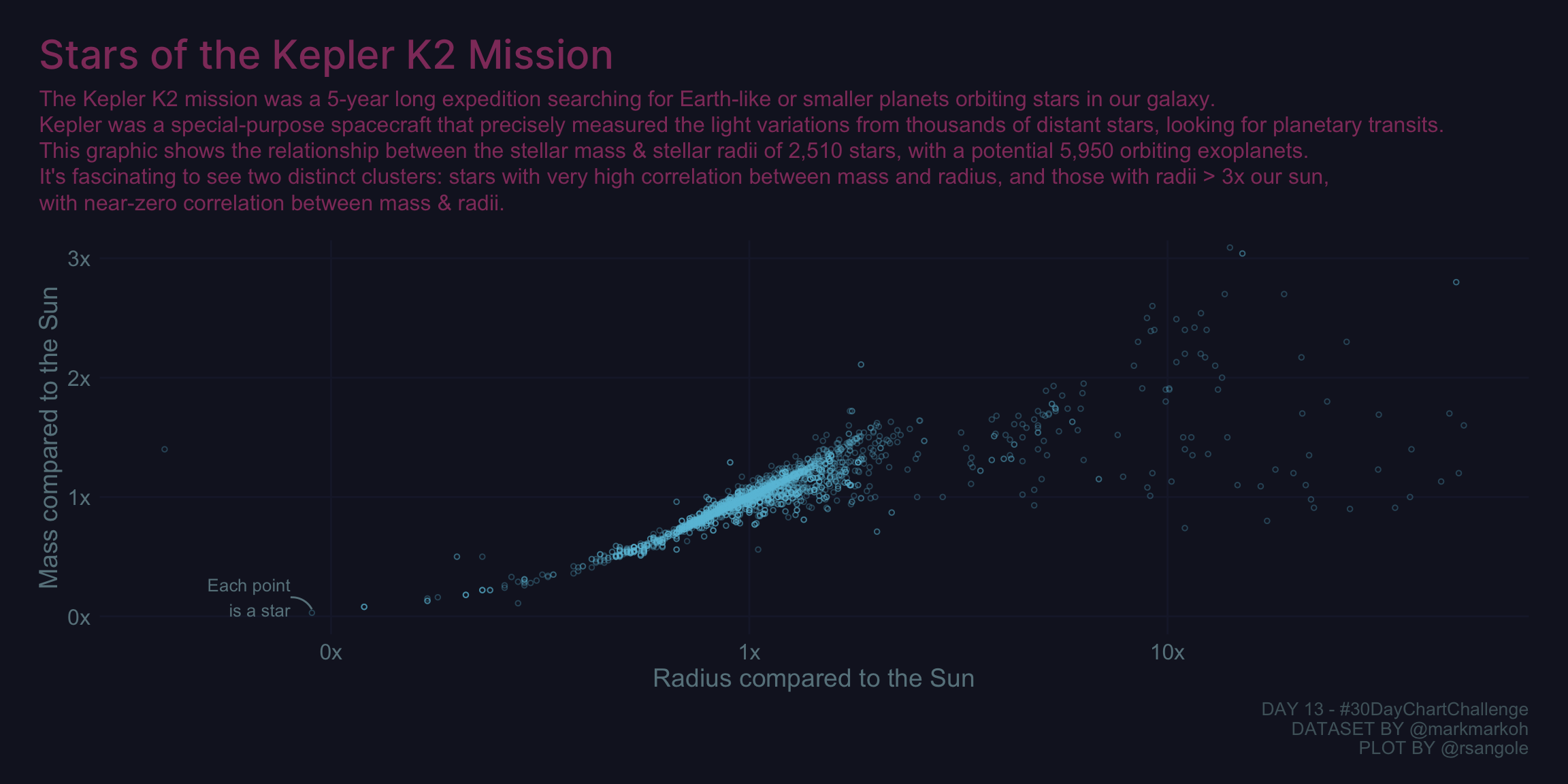
Correlation plot for Kepler’s Planets, for day 13 of the 2021 30-day-chart-challenge
library(tidyverse)
library(ggplot2)
library(ggdark)
library(ggtext)
library(ggforce)

# https://data.world/markmarkoh/kepler-confirmed-planets
dat <- data.table::fread("planets.csv")

hull_a <- dat %>%
  select(st_rad, st_mass) %>%
  filter(st_rad > 0.335 & st_rad < 2.95 & st_mass < 2) %>%
  tidyr::drop_na()
cor_a <- scales::label_number(accuracy = 0.01)(cor(hull_a)[1, 2])

hull_b <- dat %>%
  select(st_rad, st_mass) %>%
  filter(st_rad > 2.95) %>%
  tidyr::drop_na()
cor_b <- scales::label_number(accuracy = 0.01)(cor(hull_b)[1,2])

# https://coolors.co/1c1f35-151728-44243e-723054-68838c-4e636a-4ab6d3
pt_color <- "#6BC3DB"
hull_color <- "#68838C"
axis_text_color <- "#68838C"
caption_color <- "#4E636A"
grid_color <- "#1C1F35"
plot_title_color <- "#903C6A"
bg_color <- "#151728"

dat %>%
  ggplot(aes(x = st_rad, y = st_mass)) +
  geom_point(
    colour = pt_color,
    pch = 21,
    size = 1,
    alpha = 0.3
  ) +
  geom_mark_hull(
    data = hull_a,
    aes(label = glue::glue("Group A\nCorr: {cor_a}")),
    concavity = 10,
    color = hull_color,
    size = 0.3,
    radius = .02,
    con.cap = 0,
    con.colour = hull_color,
    con.border = "none",
    label.fill = bg_color,
    label.colour = hull_color,
    label.margin = margin(1, 1, 1, 1, "mm")
  ) +
  geom_mark_hull(
    data = hull_b,
    aes(label = glue::glue("Group B\nCorr: {cor_b}")),
    concavity = 10,
    color = hull_color,
    size = 0.3,
    radius = .02,
    con.cap = 0,
    con.colour = hull_color,
    con.border = "none",
    label.fill = bg_color,
    label.colour = hull_color,
    label.margin = margin(1, 1, 1, 1, "mm")
  ) +
  annotate(
    geom = "curve",
    xend = 0.09,
    yend = 0.06,
    x = 0.09 - 0.01,
    y = 0.06 + 0.1,
    curvature = -.3,
    arrow = arrow(length = unit(0, "mm")),
    color = hull_color
  ) +
  annotate(
    geom = "text",
    x = 0.09 - 0.01,
    y = 0.06 + 0.1,
    label = "Each point\nis a star",
    hjust = "right",
    size = 3.4,
    color = hull_color
  ) +
  scale_x_continuous(trans = "log10",
                     labels =
                       scales::label_number(suffix = "x",
                                            accuracy = 1,)) +
  scale_y_continuous(labels =
                       scales::label_number(suffix = "x",
                                            accuracy = 1,)) +
  dark_theme_minimal() +
  coord_cartesian(ylim = c(0, 3), clip = "off") +
  theme(
    plot.background = element_rect(color = bg_color,
                                   fill = bg_color),
    panel.grid.minor = element_blank(),
    panel.grid.major = element_line(color = grid_color),
    axis.text = element_text(size = 12, color = axis_text_color),
    axis.title.y = element_text(size = 14, color = axis_text_color),
    axis.title.x = element_text(size = 14, color = axis_text_color),
    plot.title = element_markdown(
      family = "Inter-Medium",
      color = plot_title_color,
      size = 22,
      margin = margin(0, 0, 0.5, 0, unit = "line")
    ),
    plot.title.position = "plot",
    plot.subtitle = element_markdown(
      color = plot_title_color,
      size = 12,
      lineheight = 1.2,
      margin = margin(0, 0, 1, 0, unit = "line")
    ),
    plot.margin = margin(1.5, 1.5, 1, 1.5, unit = "line"),
    legend.position = c(0.9, 0.1),
    plot.caption = element_text(colour = caption_color, size = 10)
  ) +
  labs(
    x = "Radius compared to the Sun",
    y = "Mass compared to the Sun",
    title = "Stars of the Kepler K2 Mission",
    subtitle = glue::glue("The Kepler K2 mission was a 5-year long expedition searching for Earth-like or smaller planets orbiting stars in our galaxy.<br />Kepler was a special-purpose spacecraft that precisely measured the light variations from thousands of distant stars, looking for planetary transits.<br />This graphic shows the relationship between the stellar mass & stellar radii of {n} stars, with a potential {pl_n} orbiting exoplanets.<br />It's fascinating to see two distinct clusters: stars with very high correlation between mass and radius, and those with radii > 3x our sun, <br /> with near-zero correlation between mass & radii.",
                          pl_n = scales::label_comma(accuracy = 10)(dat[,sum(pl_pnum)]),
                          n = scales::label_comma(accuracy = 10)(dat %>% count(pl_hostname) %>% nrow())),
    caption = "DAY 13 - #30DayChartChallenge\nDATASET BY @markmarkoh\nPLOT BY @rsangole"
  )