Rows: 18,387
Columns: 29
$ package <chr> "A3", "AATtools", "ABACUS", "abbreviate", "abbyyR", "abc", "abc.data", "…
$ version <chr> "1.0.0", "0.0.1", "1.0.0", "0.1", "0.5.5", "2.2.1", "1.0", "0.9.0", "1.0…
$ major <chr> "1", "0", "1", "0", "0", "2", "1", "0", "1", "1", "0", "0", "1", "1", "1…
$ minor <chr> "0", "0", "0", "1", "5", "2", "0", "9", "0", "2", "3", "15", "2", "0", "…
$ patch <chr> "0", "1", "0", NA, "5", "1", NA, "0", NA, "1", "0", "0", NA, "3", "3", N…
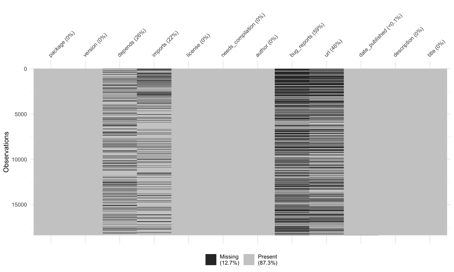
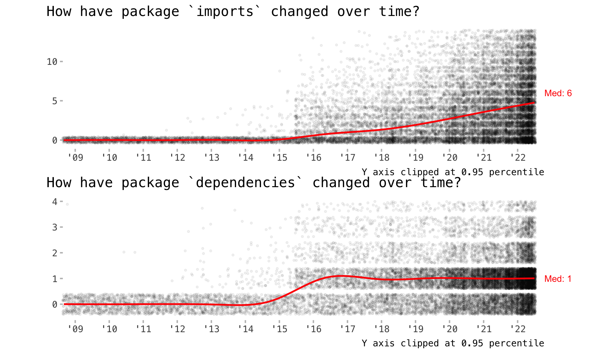
$ depends <chr> "R (>= 2.15.0), xtable, pbapply", "R (>= 3.6.0)", "R (>= 3.1.0)", NA, "R…
$ imports <chr> NA, "magrittr, dplyr, doParallel, foreach", "ggplot2 (>= 3.1.0), shiny (…
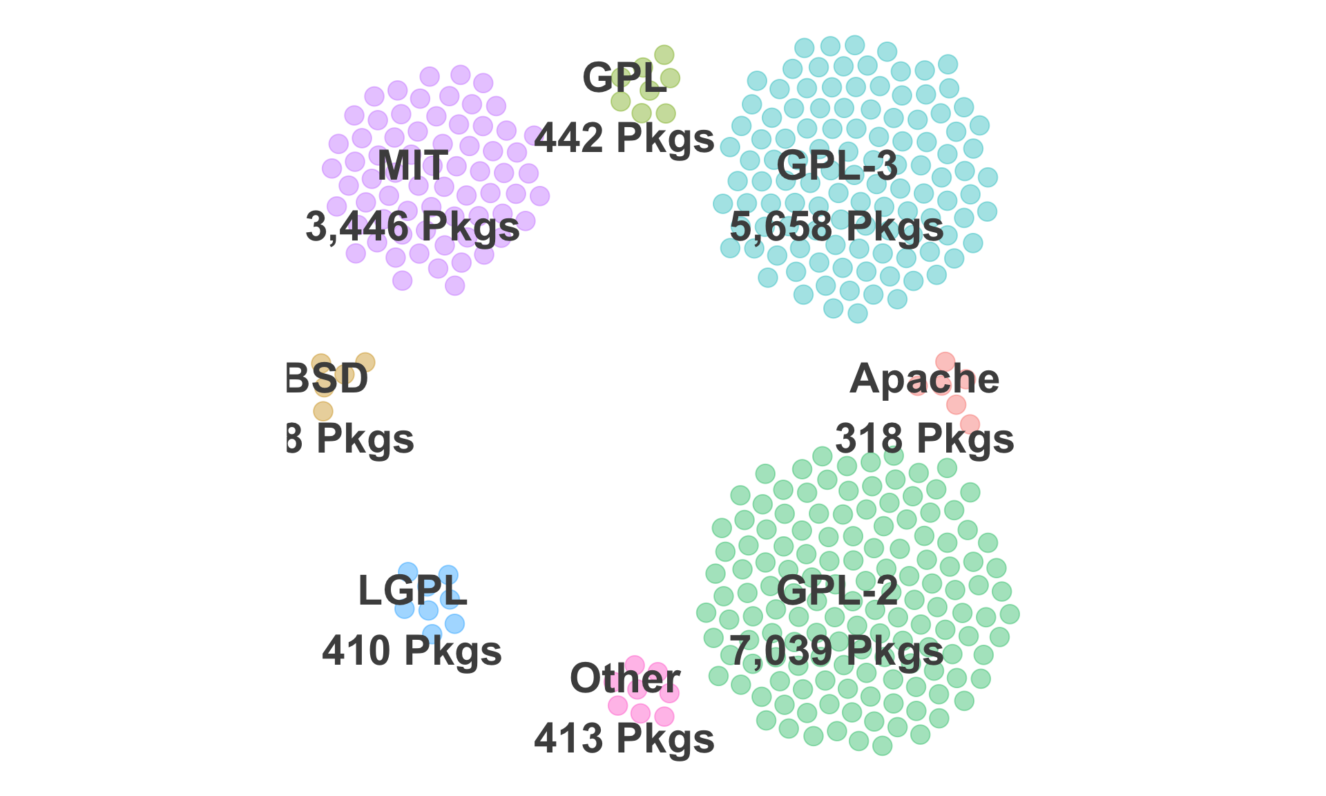
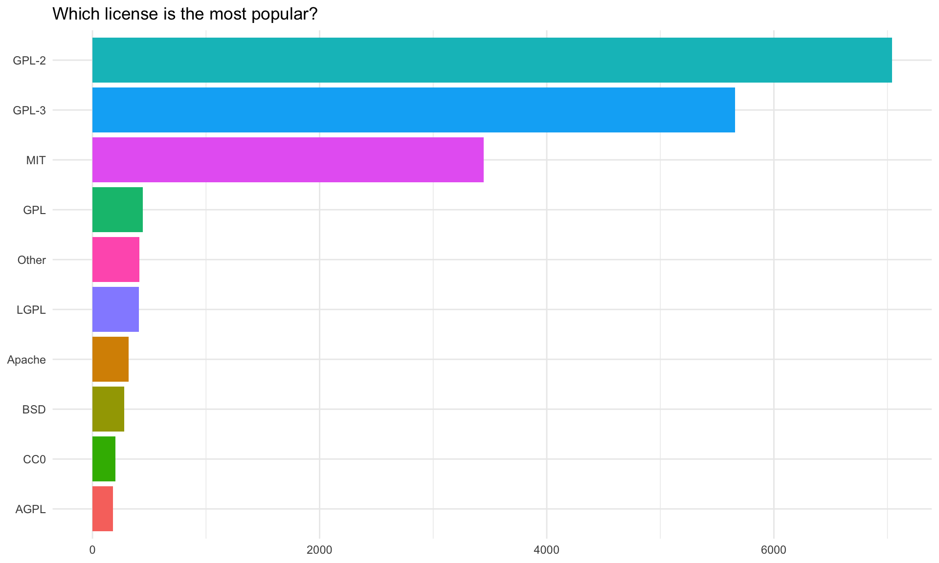
$ license <chr> "GPL (>= 2)", "GPL-3", "GPL-3", "GPL-3", "MIT + file LICENSE", "GPL (>= …
$ needs_compilation <lgl> FALSE, FALSE, FALSE, FALSE, FALSE, FALSE, FALSE, FALSE, TRUE, FALSE, TRU…
$ author <chr> "Scott Fortmann-Roe", "Sercan Kahveci [aut, cre]", "Mintu Nath [aut, cre…
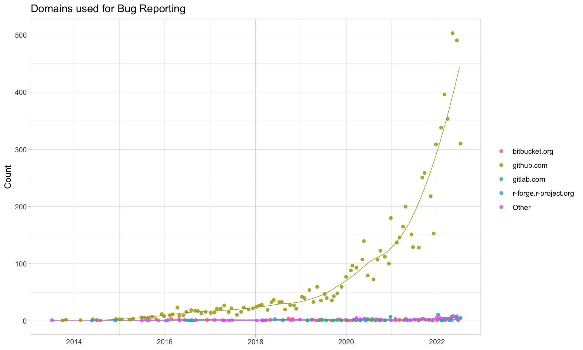
$ bug_reports <chr> NA, "https://github.com/Spiritspeak/AATtools/issues", NA, NA, "http://gi…
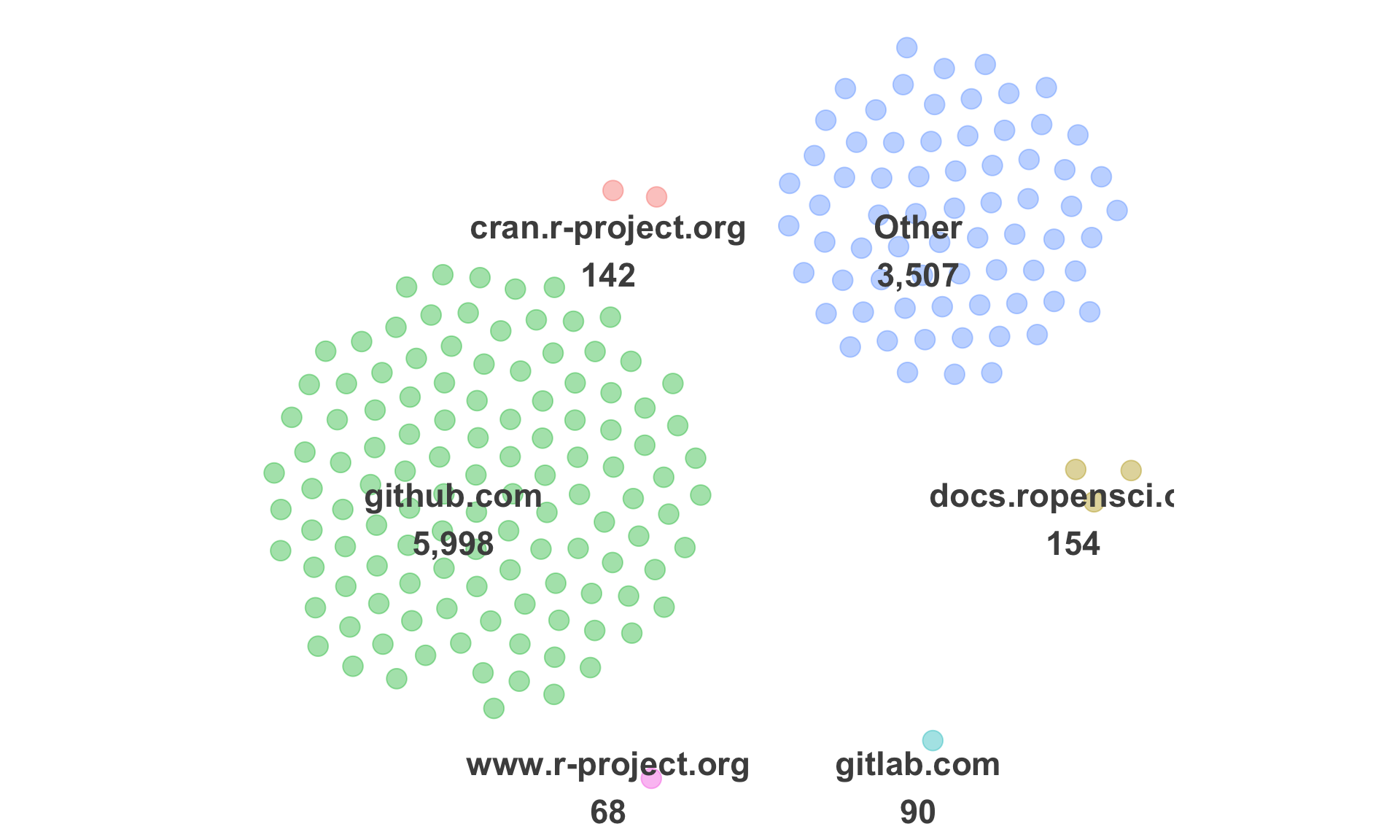
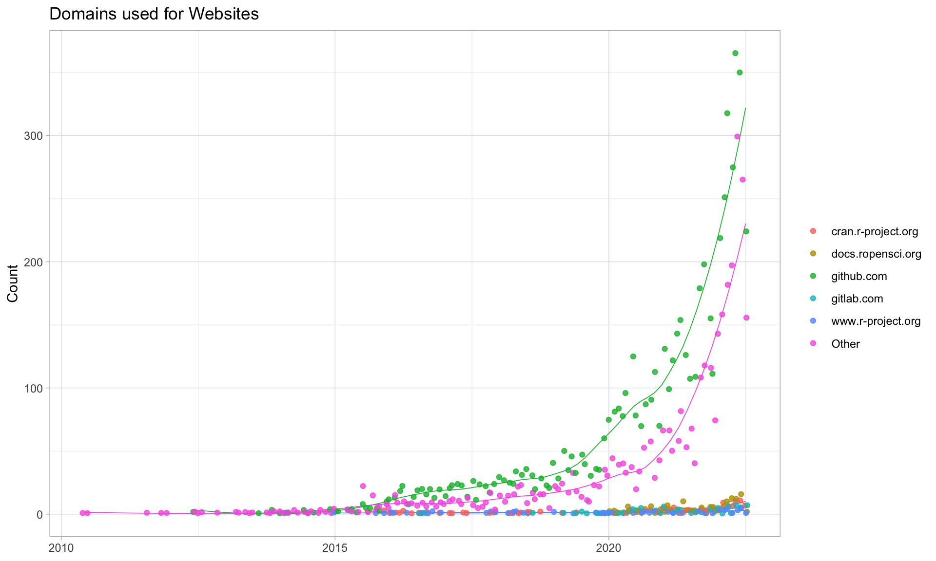
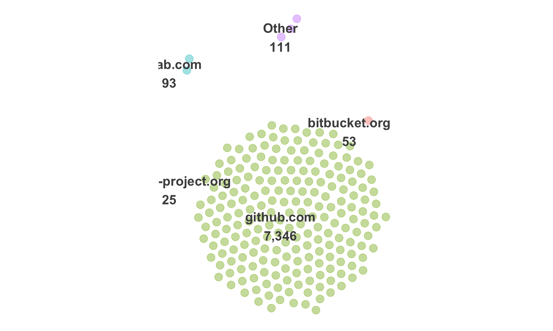
$ url <chr> NA, NA, "https://shiny.abdn.ac.uk/Stats/apps/", "https://github.com/sigb…
$ date_published <date> 2015-08-16, 2020-06-14, 2019-09-20, 2021-12-14, 2019-06-25, 2022-05-19,…
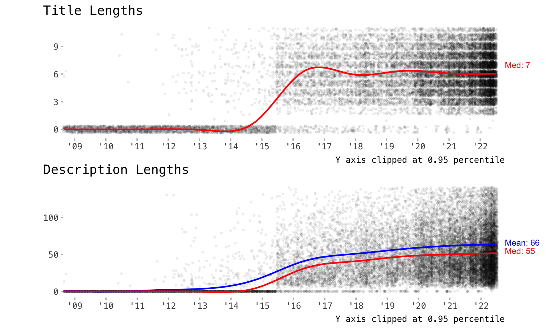
$ description <chr> "Supplies tools for tabulating and analyzing the results of predictive m…
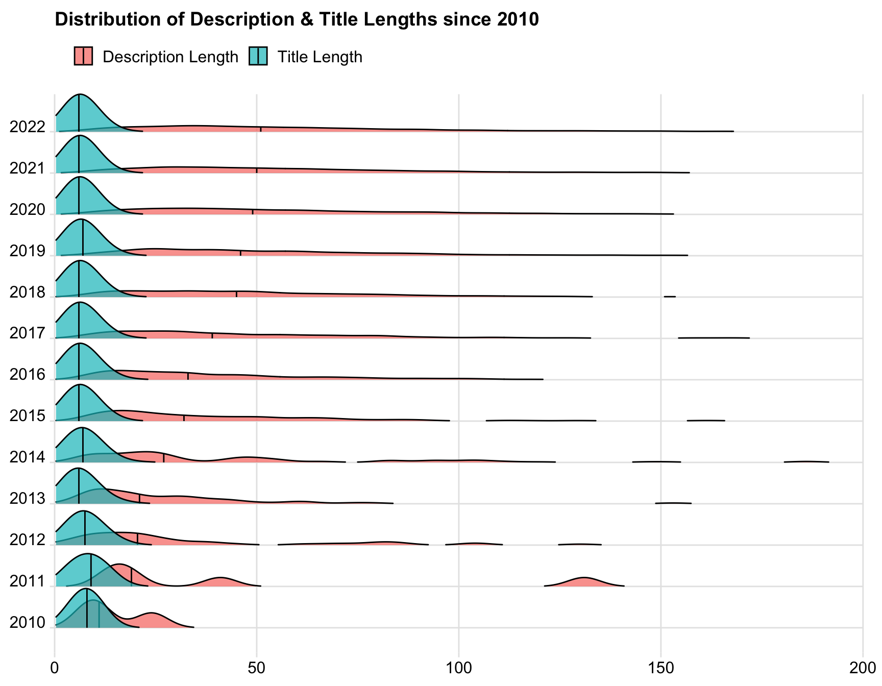
$ title <chr> "Accurate, Adaptable, and Accessible Error Metrics for Predictive\nModel…
$ num_dep <dbl> 3, 1, 1, 0, 1, 6, 1, 1, 0, 1, 1, 0, 1, 0, 6, 5, 0, 0, 1, 0, 0, 1, 1, 1, …
$ num_imports <dbl> 0, 4, 3, 0, 6, 0, 0, 3, 1, 1, 2, 4, 0, 1, 0, 0, 1, 0, 4, 4, 3, 2, 0, 8, …
$ num_authors <int> 1, 2, 2, 2, 2, 5, 5, 5, 5, 3, 3, 3, 4, 5, 4, 2, 2, 3, 14, 4, 3, 1, 6, 6,…
$ year <dbl> 2015, 2020, 2019, 2021, 2019, 2022, 2015, 2016, 2019, 2017, 2022, 2017, …
$ month <ord> Aug, Jun, Sep, Dec, Jun, May, May, Oct, Nov, Mar, May, Nov, Feb, May, Ju…
$ day <int> 16, 14, 20, 14, 25, 19, 5, 20, 13, 13, 28, 6, 4, 28, 17, 3, 20, 30, 22, …
$ wday <ord> Sun, Sun, Fri, Tue, Tue, Thu, Tue, Thu, Wed, Mon, Sat, Mon, Thu, Thu, Tu…
$ yr_mon <chr> "2015-Aug", "2020-Jun", "2019-Sep", "2021-Dec", "2019-Jun", "2022-May", …
$ dt <date> 2015-08-01, 2020-06-01, 2019-09-01, 2021-12-01, 2019-06-01, 2022-05-01,…
$ len_title <int> 9, 9, 8, 3, 8, 6, 8, 6, 9, 3, 5, 7, 7, 7, 4, 5, 5, 3, 4, 4, 5, 3, 8, 11,…
$ len_desc <int> 28, 24, 40, 21, 52, 36, 11, 32, 41, 163, 19, 56, 33, 89, 12, 25, 88, 65,…
$ license_cleaned <chr> "GPL-2", "GPL-3", "GPL-3", "GPL-3", "MIT", "GPL-3", "GPL-3", "GPL-3", "G…
$ url_domain <chr> NA, NA, "shiny.abdn.ac.uk", "github.com", "github.com", NA, NA, NA, NA, …
$ bug_domain <chr> NA, "github.com", NA, NA, "github.com", NA, NA, NA, NA, NA, "github.com"…