Performance Benchmarking for Dummy Variable Creation

How do the four popular methods of creating dummy variables perform on large datasets? Let’s find out!

Motivation

Very recently, at work, we got into a discussion about creation of dummy variables in R code. We were dealing with a fairly large dataset of roughly 500,000 observations for roughly 120 predictor variables. Almost all of them were categorical variables, many of them with a fairly large number of factor levels (think 20-100). The types of models we needed to investigate required creation of dummy variables (think xgboost). There are a few ways to convert categoricals into dummy variables in R. However, I did not find any comparison of performance for large datasets.

So here it goes.

Why do we need dummy variables?

I won’t say any more here. Plenty of good resources on the web: here, here, and here.

Ways to create dummy variables in R

These are the methods I’ve found to create dummy variables in R. I’ve explored each of these

• stats::model.matrix()
• dummies::dummy.data.frame()
• dummy::dummy()
  
• caret::dummyVars()

Prepping some data to try these out. Using the HairEyeColor dataset as an example. It consists of 3 categorical vars and 1 numerical var. Perfect to try things out. Adding a response variable Y too.

library(dplyr)
library(readr)
library(purrr)
library(magrittr)
data("HairEyeColor")
HairEyeColor %<>% tbl_df()
HairEyeColor$Y = sample(c(0,1),dim(HairEyeColor)[1],replace = T) %>% factor(levels = c(0,1),labels = c('No','Yes'))
glimpse(HairEyeColor)

Rows: 32
Columns: 5
$ Hair <chr> "Black", "Brown", "Red", "Blond", "Black", "Brown", "Red", "Blond…
$ Eye  <chr> "Brown", "Brown", "Brown", "Brown", "Blue", "Blue", "Blue", "Blue…
$ Sex  <chr> "Male", "Male", "Male", "Male", "Male", "Male", "Male", "Male", "…
$ n    <dbl> 32, 53, 10, 3, 11, 50, 10, 30, 10, 25, 7, 5, 3, 15, 7, 8, 36, 66,…
$ Y    <fct> Yes, Yes, Yes, No, Yes, No, Yes, No, Yes, No, No, Yes, No, No, Ye…

Let’s look at each package:

stats package

The stats package has a function called model.matrix which converts factor variables to dummy variables. It also drops the response variable.

Some pros

• Works with tibbles
• Really fast
• Retains numerical columns as is
• Formula interface allows one to specify what Y is

Some cons

• Need to add the response Y back into the mix, if we need it

head(model.matrix(Y~.-1,HairEyeColor),3)

  HairBlack HairBlond HairBrown HairRed EyeBrown EyeGreen EyeHazel SexMale  n
1         1         0         0       0        1        0        0       1 32
2         0         0         1       0        1        0        0       1 53
3         0         0         0       1        1        0        0       1 10

dummies package

dummies has a command called dummy.data.frame which does the needful.

Some pros

• Retains numerical columns as is
• Can create based dummy variables for numeric columns too

Some cons

• Doesn’t work with tibbles
• Doesn’t have a formula interface to specify what Y is. Need to manually remove response variable from dataframe

library(dummies)
head(dummy.data.frame(data = as.data.frame(HairEyeColor),sep="."),3)

  Hair.Black Hair.Blond Hair.Brown Hair.Red Eye.Blue Eye.Brown Eye.Green
1          1          0          0        0        0         1         0
2          0          0          1        0        0         1         0
3          0          0          0        1        0         1         0
  Eye.Hazel Sex.Female Sex.Male  n Y.No Y.Yes
1         0          0        1 32    0     1
2         0          0        1 53    0     1
3         0          0        1 10    0     1

dummy package

dummy creates dummy variables of all the factors and character vectors in a data frame. It also supports settings in which the user only wants to compute dummies for the categorical values that were present in another data set. This is especially useful in the context of predictive modeling, in which the new (test) data has more or other categories than the training data. ¹

Some pros

• Works with tibbles
• Retains numerical columns as is
• Can create based dummy variables for numeric columns too
• p parameter can select terms in terms of frequency
• Can grab only those variables in a separate dataframe
• Can create based dummy variables for numeric columns too

Some cons

• Doesn’t have a formula interface to specify what Y is. Need to manually remove response variable from dataframe

library(dummy)
head(dummy(HairEyeColor),3)

  Hair_Black Hair_Blond Hair_Brown Hair_Red Eye_Blue Eye_Brown Eye_Green
1          1          0          0        0        0         1         0
2          0          0          1        0        0         1         0
3          0          0          0        1        0         1         0
  Eye_Hazel Sex_Female Sex_Male Y_No Y_Yes
1         0          0        1    0     1
2         0          0        1    0     1
3         0          0        1    0     1

Side note: there’s a useful feature to grab all the categories in a factor variable.

categories(HairEyeColor)

$Hair
[1] "Black" "Blond" "Brown" "Red"  

$Eye
[1] "Blue"  "Brown" "Green" "Hazel"

$Sex
[1] "Female" "Male"  

$Y
[1] "No"  "Yes"

caret package

Lastly, there’s the caret package’s dummyVars(). This follows a different paradigm. First, we create reciepe of sorts, which just creates an object that specifies how the dataframe gets dummy-fied. Then, use the predict() to make the actual conversions.

Some pros

• Works on creating full rank & less than full rank matrix post-conversion
• Has a feature to keep only the level names in the final dummy columns
• Can directly create a sparse matrix
• Retains numerical columns as is

Some cons

• Y needs a factor
• If the cateogical variables aren’t factors, you can’t use the sep=' ' feature

library(caret)
HairEyeColor$Hair <- as.factor(HairEyeColor$Hair)
HairEyeColor$Eye <- as.factor(HairEyeColor$Eye)
HairEyeColor$Sex <- as.factor(HairEyeColor$Sex)
dV <- dummyVars(formula = Y~.,data = HairEyeColor)
dV

Dummy Variable Object

Formula: Y ~ .
5 variables, 4 factors
Variables and levels will be separated by '.'
A less than full rank encoding is used

head(predict(object = dV, newdata = HairEyeColor),3)

  Hair.Black Hair.Blond Hair.Brown Hair.Red Eye.Blue Eye.Brown Eye.Green
1          1          0          0        0        0         1         0
2          0          0          1        0        0         1         0
3          0          0          0        1        0         1         0
  Eye.Hazel Sex.Female Sex.Male  n
1         0          0        1 32
2         0          0        1 53
3         0          0        1 10

Performance comparison

I’ve run these benchmarks on my Macbook Pro with these specs:

• Processor Name: Intel Core i5
• Processor Speed: 2.4 GHz
• Number of Processors: 1
• Total Number of Cores: 2
• L2 Cache (per Core): 256 KB
• L3 Cache: 3 MB
• Memory: 8 GB

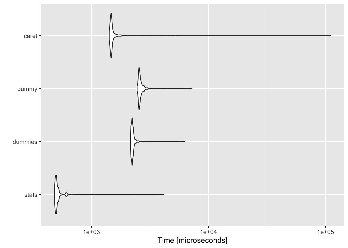
Smaller datasets

The first dataset used is the HairEyeColor. 32 rows, 1 numeric var, 3 categorical var. All the resulting dataframes are as similar as possible… they all retain the Y variable at the end.

library(microbenchmark)
HairEyeColor_df <- as.data.frame(HairEyeColor)

stats_fn <- function(D){
    stats::model.matrix(Y~.-1,D) %>% 
        cbind(D$Y)
}

dummies_fn <- function(D){
    dummies::dummy.data.frame(D[,-5]) %>% 
        cbind(D$Y)
}

dummy_fn <- function(D){
    dummy::dummy(D[,-5]) %>% 
        cbind(D$Y)
}

caret_fn <- function(D){
    dV <- caret::dummyVars(formula = Y~.,data = D)
    predict(object = dV, newdata = D) %>% 
        cbind(D$Y)
    }

microbenchmark::microbenchmark(
    stats = stats_fn(D = HairEyeColor),
    dummies = dummies_fn(D = HairEyeColor_df),
    dummy = dummy_fn(D = HairEyeColor),
    caret = caret_fn(D = HairEyeColor),
    times = 1000L,
    control = list(order = 'block'),
    unit = 's'
    ) -> benchmarks

autoplot(benchmarks)

The results speak for themself. The stats is clearly the fastest with dummies and caret being a more distant 2nd & 3rd.

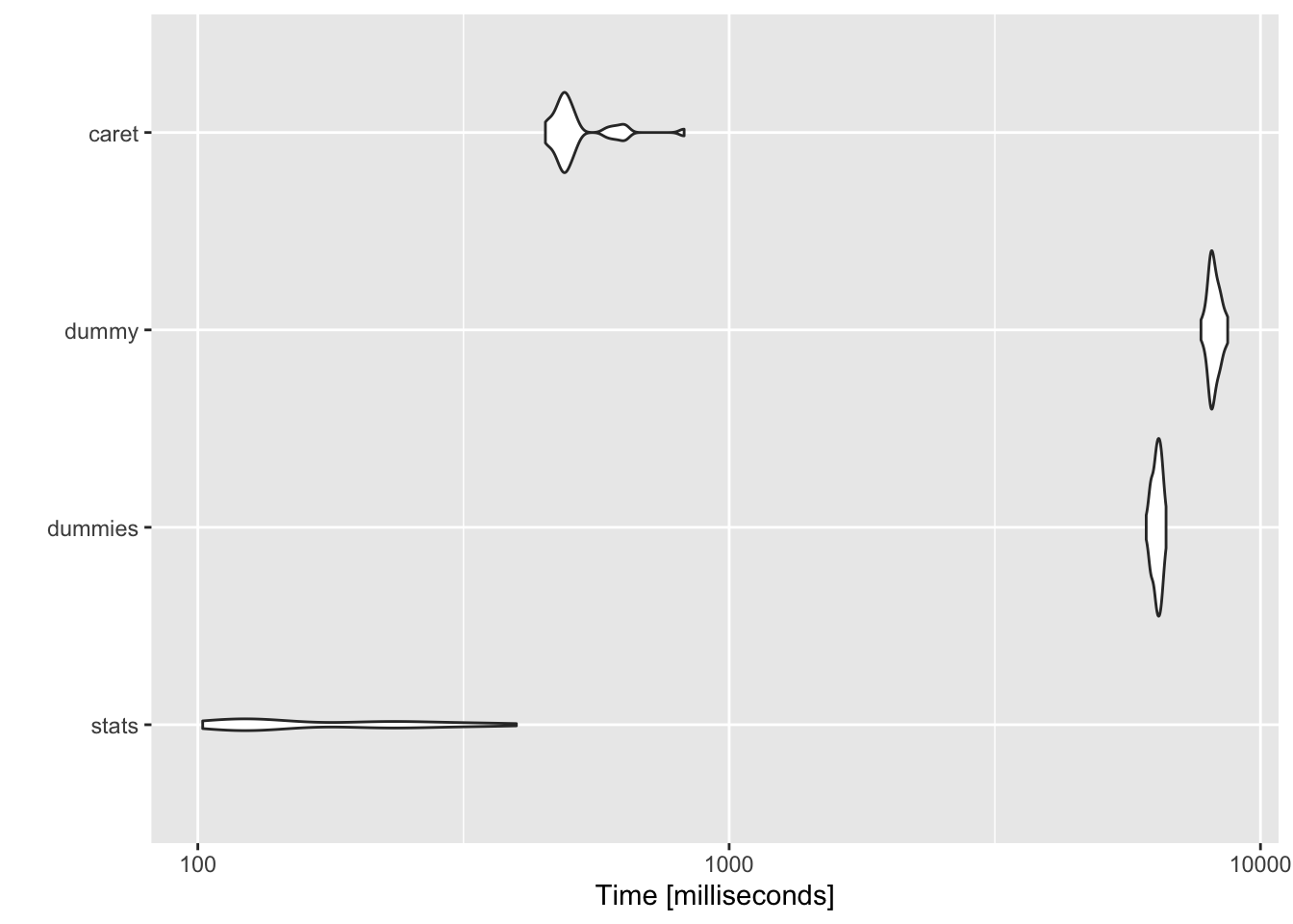
Large datasets

To leverage a large dataset for this analysis, I’m using the Accident & Traffic Flow dataset, which is fairly big - 570,011 rows and 33 columns. I’ve narrowed down to 7 categorical variables to test the packages, and I’ve created a fake response variable as well.

data <- read_csv('~/github/github.com/blog-large-data/accidents_2005_to_2007.csv',progress = F)
data %<>%
    transmute(
        Day_of_Week = as.factor(Day_of_Week),
        Road_Type = Road_Type %>% stringr::str_replace_all('[()/ ]','.') %>% as.factor,
        Weather = Weather_Conditions %>% stringr::str_replace_all('[()/ ]','.') %>% as.factor,
        RoadSurface = Road_Surface_Conditions %>% stringr::str_replace_all('[()/ ]','.') %>% as.factor,
        PedHC =  `Pedestrian_Crossing-Human_Control` %>% stringr::str_replace_all('[()/ ]','.') %>% as.factor,
        PedPF =  `Pedestrian_Crossing-Physical_Facilities` %>% stringr::str_replace_all('[()/ ]','.') %>% as.factor,
        Year =  as.factor(Year)
    ) %>% 
    mutate(
        Y = sample(c(0,1),dim(data)[1],replace = T) %>% factor(levels = c(0,1),labels = c('No','Yes'))
    )
dim(data)

[1] 570011      8

In total, there will be 39 dummy variable columns created for these 7 factor variables, as we can see here:

map_int(data,~length(levels(.x)))

Day_of_Week   Road_Type     Weather RoadSurface       PedHC       PedPF 
          7           6           9           5           3           6 
       Year           Y 
          3           2 

Now for the benchmarks:

data_df <- as.data.frame(data)
stats_fn <- function(D){
    stats::model.matrix(Y~.-1,D) %>% 
        cbind(D$Y)
}

dummies_fn <- function(D){
    dummies::dummy.data.frame(D[,-8]) %>% 
        cbind(D$Y)
}

dummy_fn <- function(D){
    dummy::dummy(D[,-8]) %>% 
        cbind(D$Y)
}

caret_fn <- function(D){
    dV <- caret::dummyVars(formula = Y~.,data = D)
    predict(object = dV, newdata = D) %>% 
        cbind(D$Y)
    }

microbenchmark::microbenchmark(
    stats = stats_fn(D = data),
    dummies = dummies_fn(D = data_df),
    dummy = dummy_fn(D = data),
    caret = caret_fn(D = data),
    times = 30L,
    control = list(order = 'block')
    ) -> benchmarks

autoplot(benchmarks)

Just like before, stats is clerly the fastest.

Conclusion

• Stick to stats::model.matrix(). It works with tibbles, it’s fast, and it takes a formula.
• If you like the caret package and it’s interface, it’s the 2nd best choice.
• dummy or dummies doesn’t seem to offer any advantages to these packages.

Qs

• Are there other packages you recommend for dummy variable creation? If yes, please let me know in the comments.
• Could you run the bench marks on more powerful machines and larger datasets, and share your results? I’d like to append them here.

Footnotes

1. Straight from the dummy help file