TidyTuesday

Visualization

Author

Rahul

Published

January 11, 2021

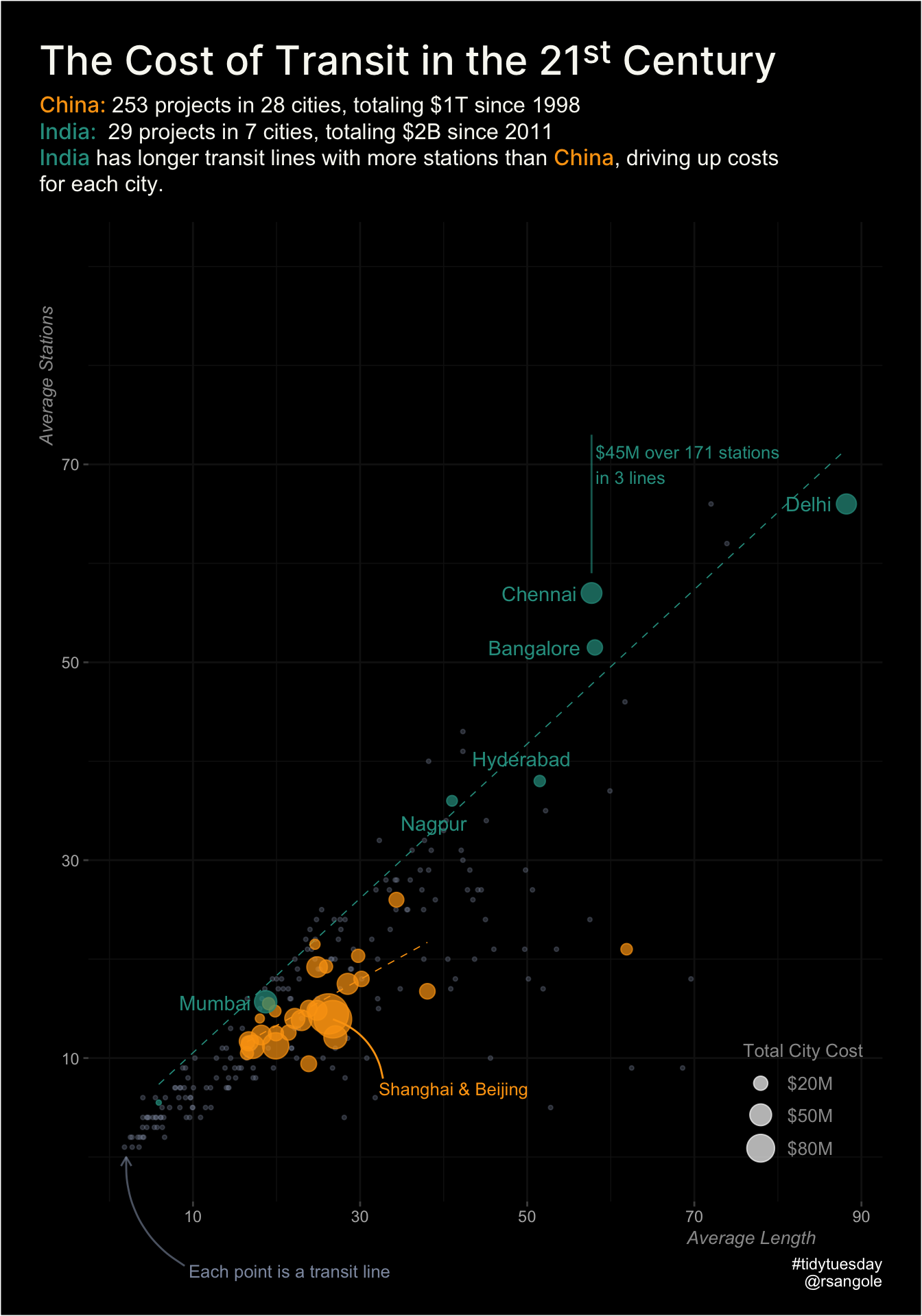
Comparing Indian rail projects to our neighbour China, I find that, on average, Indian lines have a higher number of stations and longer lines than our Chinese counterparts.

Also, number of stations to track length is amazingly linear (duh).#TidyTuesday #rstats #dataviz pic.twitter.com/pL4eYBIKNE
— Rahul (@rsangole) January 10, 2021

library(tidyverse)
library(ggplot2)
library(ggrepel)
library(ggdark)
library(ggtext)

transit_cost <- data.table::fread("transit_cost.csv")

transit_cost <- transit_cost %>%
  mutate(tunnel_per = as.numeric(str_replace(tunnel_per, "%", "")),
         real_cost = as.numeric(real_cost),
         country = ifelse(is.na(country), "Unk", country),
         cc_id = paste(country,city))

dat <- transit_cost %>%
  group_by(country, city) %>%
  summarise(
    total_projects = n(),
    total_stations = sum(stations, na.rm = TRUE),
    total_tunnel_len = sum(tunnel, na.rm = TRUE),
    total_len = sum(length, na.rm = TRUE),
    tunnel_pc = total_tunnel_len/total_len,
    total_cost = sum(real_cost, na.rm = TRUE) / 1e3, #now in Billions
    avg_stations = mean(stations, na.rm = TRUE),
    avg_tunnel_len = mean(tunnel, na.rm = TRUE),
    avg_len = mean(length, na.rm = TRUE),
    tunnel_pc = avg_tunnel_len/avg_len,
    avg_cost = mean(real_cost, na.rm = TRUE)
  ) %>%
  filter(total_len < 10000,
         total_projects > 1,
         country %in% c("CN", "IN")) %>%
  mutate(cc_id = paste(country,city),
         country = ifelse(country == "CN", "China", "India"))
glimpse(dat)

Rows: 35
Columns: 13
Groups: country [2]
$ country          <chr> "China", "China", "China", "China", "China", "China",…
$ city             <chr> "Beijing", "Changchun", "Changsha", "Chengdu", "Chong…
$ total_projects   <int> 27, 7, 13, 11, 11, 7, 3, 10, 5, 11, 10, 8, 2, 5, 12, …
$ total_stations   <int> 376, 81, 152, 152, 163, 66, 61, 121, 90, 154, 192, 10…
$ total_tunnel_len <dbl> 450.0686, 95.5000, 164.5400, 225.1000, 156.3370, 151.…
$ total_len        <dbl> 721.973, 116.000, 216.860, 252.950, 273.220, 166.940,…
$ tunnel_pc        <dbl> 0.7650659, 0.8232759, 0.8219666, 0.8898992, 0.7867776…
$ total_cost       <dbl> 138.86373, 16.92127, 38.33016, 44.59756, 41.87035, 25…
$ avg_stations     <dbl> 13.925926, 11.571429, 11.692308, 13.818182, 14.818182…
$ avg_tunnel_len   <dbl> 20.45766, 13.64286, 13.71167, 20.46364, 19.54213, 21.…
$ avg_len          <dbl> 26.73974, 16.57143, 16.68154, 22.99545, 24.83818, 23.…
$ avg_cost         <dbl> 5143.101, 2417.324, 2948.474, 4054.324, 3806.395, 364…
$ cc_id            <chr> "CN Beijing", "CN Changchun", "CN Changsha", "CN Chen…

label_dat_india <- dat %>%
  filter(country %in% "India",
         city != "Gurgaon")
label_dat_china <- dat %>%
  filter(city %in% c("Shanghai", "Beijing"))

to_plot <- transit_cost %>%
  tidyr::drop_na() %>%
  filter(cc_id %in% dat$cc_id,
         country %in% c("CN", "IN"),
         length < 100) %>%
  mutate(country = ifelse(country == "CN", "China", "India"))

in_color <- "#2a9d8f"
cn_color <- "#fca311"

chennai <- dat %>% filter(city == "Chennai")
chennai_stations <- chennai$total_stations
chennai_projects <- chennai$total_projects
chennai_x <- chennai$avg_len
chennai_y <- chennai$avg_stations
chennai_cost <- chennai$total_cost

to_plot %>%
  ggplot(aes(length, stations)) +
  geom_point(color = "#8d99ae", size = 0.8, show.legend = FALSE, alpha = 0.3) +
  geom_smooth(data = dat %>% filter(city!="Wenzhou"),
              aes(avg_len, avg_stations, color = country),
              se=FALSE, linetype="dashed", size=0.3, method = "lm", span = 4) +
  geom_point(data = dat,
             aes(avg_len, avg_stations, color = country, size = total_cost^1.3),
             pch = 19, alpha = 0.7) +
  geom_text_repel(data = label_dat_india,
                   aes(avg_len, avg_stations,
                                   label = city,
                                   color = country),
                                   min.segment.length = 1,
                   box.padding = unit(0.5, "line"),
                   nudge_x = -1,
                   show.legend = FALSE) +
  annotate(geom = "curve",
           xend = label_dat_china$avg_len[1], yend = label_dat_china$avg_stations[1],
           x = label_dat_china$avg_len[1] + 6, y = label_dat_china$avg_stations[1] - 6,
           curvature = .3, arrow = arrow(length = unit(0, "mm")), color = "#fca311") +
  annotate(geom = "text",
           x = label_dat_china$avg_len[1] + 5.5, y = label_dat_china$avg_stations[1] - 7,
           label = "Shanghai & Beijing", hjust = "left", size = 3.4, color = "#fca311") +
  annotate(geom = "curve",
           xend = 2, yend = 0,
           x = 2 + 7, y = 0 - 11,
           curvature = -.3, arrow = arrow(length = unit(2, "mm")), color = "#8d99ae", alpha = 0.6) +
  annotate(geom = "text",
           x = 2 + 7.5, y = 0 - 11.5,
           label = "Each point is a transit line", hjust = "left", size = 3.4, color = "#8d99ae") +
  annotate(geom = "curve",
           xend = chennai_x, yend = chennai_y + 2,
           x = chennai_x, y = chennai_y + 16,
           curvature = 0, arrow = arrow(length = unit(0, "mm")), color = in_color, alpha = 0.6) +
  annotate(geom = "text",
           x = chennai_x + 0.5, y = chennai_y + 13,
           label = glue::glue(
             "{cost} over {stations} stations
             in {chennai_projects} lines",
             x = scales::label_number(accuracy = 1, suffix = " km")(chennai_x),
             y = chennai_y,
             stations = chennai_stations,
             chennai_projects = chennai_projects,
             cost = scales::label_dollar(accuracy = 1, suffix = "M")(chennai_cost)
             ),
           hjust = "left", size = 3.4, color = in_color) +
  dark_theme_minimal() +
  scale_x_continuous(breaks = seq(10, 90, 20)) +
  scale_y_continuous(breaks = seq(10, 70, 20)) +
  scale_size(name = "Total City Cost",
             breaks = c(20^1.3, 50^1.3, 80^1.3),
             labels = c("$20M", "$50M","$80M"),
             range = c(1,10)
             ) +
  coord_cartesian(ylim = c(0,90), clip = "off") +
  labs(
    title = "The Cost of Transit in the 21<sup>st</sup> Century",
    subtitle = glue::glue("<span style='color:{cn_color};font-family:Inter-Medium;'>China: </span>253 projects in 28 cities, totaling $1T since 1998<br /><span style='color:{in_color};font-family:Inter-Medium;'>India: </span> 29 projects in 7 cities, totaling $2B since 2011<br /><span style='color:{in_color};font-family:Inter-Medium;'>India</span> has longer transit lines with more stations than <span style='color:{cn_color};font-family:Inter-Medium;'>China</span>, driving up costs <br />for each city."),
    x = "Average Length",
    y = "Average Stations",
    caption = "#tidytuesday\n@rsangole"
    ) +
  theme(
    legend.title = element_text(size = 10, color = "gray60"),
    legend.text =  element_text(size = 10, color = "gray60"),
    axis.ticks.x.bottom = element_line(colour = "gray30",size = 0.5),
    axis.ticks.y.left = element_line(colour = "gray30"),
    axis.title.y = element_text(hjust = .9, size = 10, face = "italic", color = "gray60"),
    axis.title.x = element_text(hjust = .9, size = 10, face = "italic", color = "gray60"),
    plot.title = element_markdown(family = "Inter-Medium", color = "#f8f8f2", size = 22,
                                  margin = margin(0, 0, 0.5, 0, unit = "line")),
    plot.title.position = "plot",
    plot.subtitle = element_markdown(color = "#f8f8f2", size = 12, lineheight = 1.2,
                                     margin = margin(0, 0, 1, 0, unit = "line")),
    plot.margin = margin(1.5, 1.5, 1, 1.5, unit = "line"),
    legend.position = c(0.9,0.1)
    ) +
  scale_discrete_manual(aesthetics = "color",
                        values = c("India" = in_color, "China" = cn_color),
                        guide = F)